How To Label
Labeling independent components (ICs) on this site based on their displayed properties is relatively easy once you understand what information the images provide and what the buttons at the bottom of each IC properties page represent.
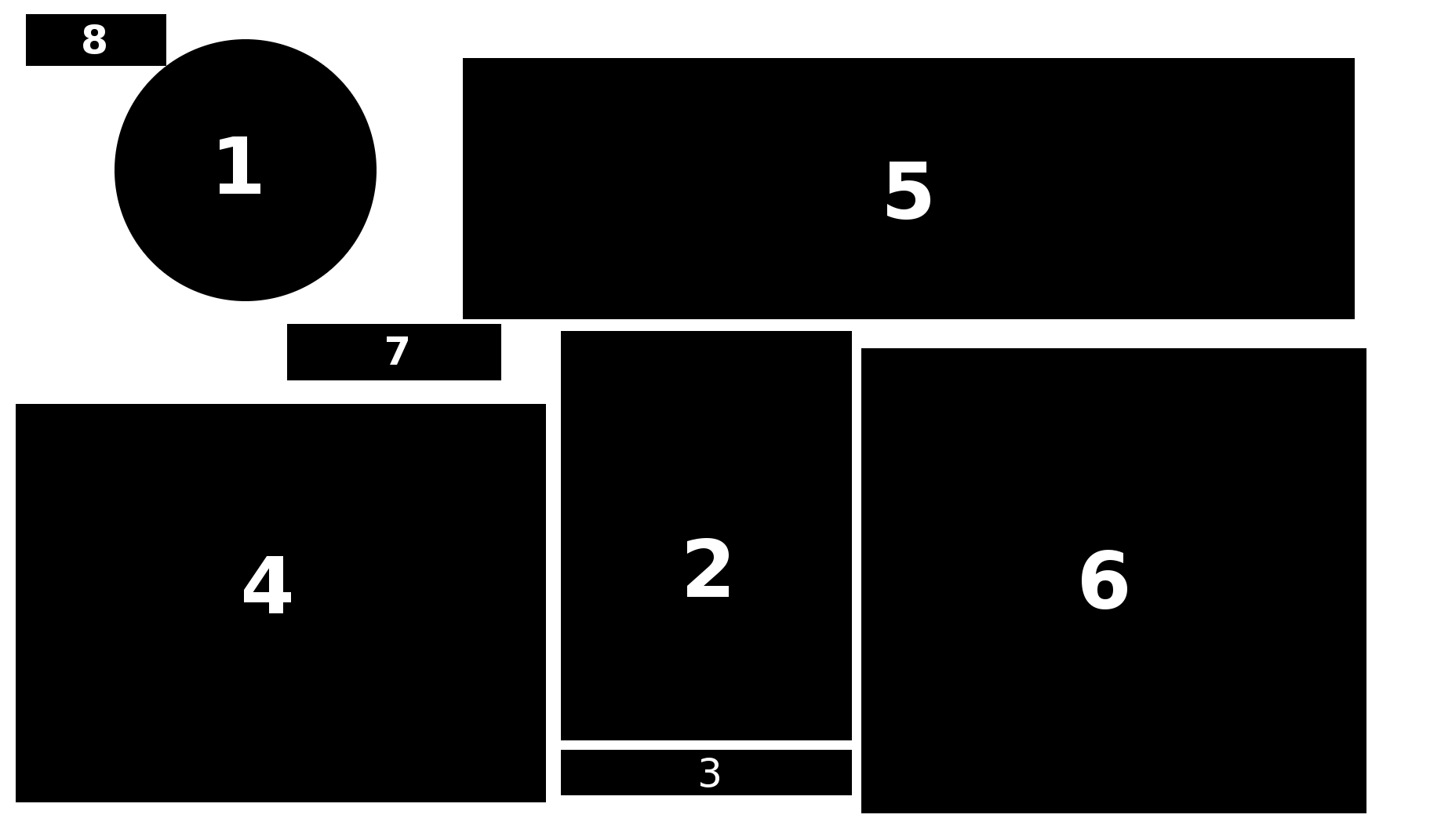
Assigning Labels
Instead of assigning individual labels to a component, you may assign as many labels as you want to a component. While this initially makes the process of labeling more confusing, we believe the added ability to express uncertainty is worth the increase in complexity.
Possible labels include:
- Brain
- Eye
- Muscle
- Heart
- Line Noise
- Channel Noise
- Other
- ?
There are four different ways to label components. Choose the method you feel is appropriate based on how confident you are in your decision.
- If you are sure of a label, mark only that one and then click "Next."
- If you can't tell between two or three categories, but you are sure it's one of them, then mark all of those and click "Next."
- If (as in case #2 above) you mark a few candidate classes, but also fear you may be wrong about these, click the "?" marker as well to show this uncertainty.
- If you don't know what the component type is, then mark only "?" and click "Next."
A note on "Other" vs "?": Marking "Other" means that you believe the component does not have an inherent meaning (or possibly one that we did not make a category for) whereas marking "?" means that you are uncertain as to the accuracy of the categories you have marked. Please, do not feel hesitation in marking "?". Many components are difficult to classify and knowing which ones are confusing is helpful.
Hotkeys: Instead of clicking buttons, you can also use the keyboard. Press keys '1' to '8' to add labels in the order of the buttons (e.g. 1 for "Brain", 4 for "Heart", and 8 for "?"). Press Enter to submit your label and move on to the next component.
Reading The Images
Here are two example image:
  |
 |
Each IC properties image has the following information:
-
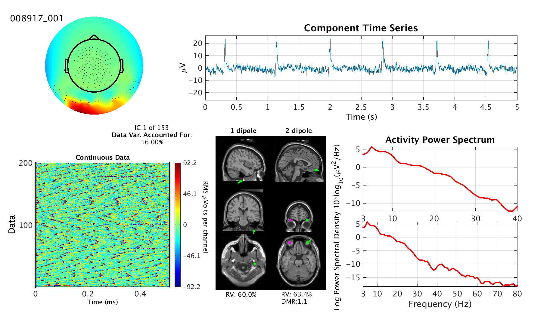
Scalp Topography (image at the top/left): Looks like a colorful swath over a cartoon head with black dots
that represent electrode positions. This shows what effect the independent component process has on each electrode.
Green represents no effect, where red and blue show positive and negative contributions, respectively.
Note: colors far from any electrodes are susceptible to interpolation/extrapolation artifacts. See the top left image
for an example.
Summary:
- Shows effects of component activity on the electrodes.
- Be wary of channel extrapolation/interpolation artifacts.
-
Dipole Model Plot (middle bottom): Shows the estimated locations of brain equivalent current dipoles (ECD) best
fitting the IC scalp topography for models using one dipole (left) and two bilaterally symmetric dipoles (right).
To elaborate, an ECD is modeled in the head by placing it with the
correct position and orientation to best recreate the scalp topography. A model with one dipole is shown in the
left column, two dipoles in the right column. The top row shows a sagittal MRI image at the estimated location of the
dipole (halfway between the dipoles in the right column). The middle row shows the same but with a coronal slice and
the bottom row with an axial slice. The assumption of an ECD source does not always hold. Therefore, just because
a location is shown does not mean it is accurate or meaningful.
Summary:
- Shows estimated location of the source of the component.
- The left column shows the best-fitting single dipole model, the right shows the best-fitting model with two bilaterally symmetric dipoles (position symmetric but not necessarily orientation symmetric).
- Source locations shown are not always accurate, as the underlying model assumptions may not apply.
-
Residual Variance (RV) and Dipole Moment Ratio (DMR) (below dipole plot): RV tells how much variance
in the scalp topography is left over after subtracting the projected topography of the model equivalent
current dipole(s) from the IC scalp topography. This value provides
a measure of how "dipolar" the scalp topography is. There are situations when the topography requires two dipoles to
be accurately modeled, and can therefore produce high residual variance for a "one dipole" fit even though the
ECD generator assumption still fits. For this reason, we include the residual variance for both "one dipole" and
"two dipole fits." Two dipoles should always provide a lower value for residual variance, as when the second is
not required, it will simply model some of the noise/errors in the electrical forward problem head model used
and/or in the ICA decomposition. DMR is the ratio of moments (lengths/magnitudes) of the dipoles in the two-dipole
model. It provides an easy way to determine if the second dipole has any meaningful effect. If the DMR is one,
then the two dipoles have equal effect. If the DMR is much larger than one, then the weaker of the two dipoles is negligible.
Summary:
- RV is a measure of how "dipolar" (i.e., well fit by an equivalent dipole model) a component is.
- Two dipoles will (almost) always provide a lower RV than one dipole. Fitting a 2nd dipole (even a bilaterally symmetric one) can nearly always "clean up" some (always present) error in the forward head model or decomposition.
- Most components are not dipolar. Of those that are, the majority require only one dipole.
-
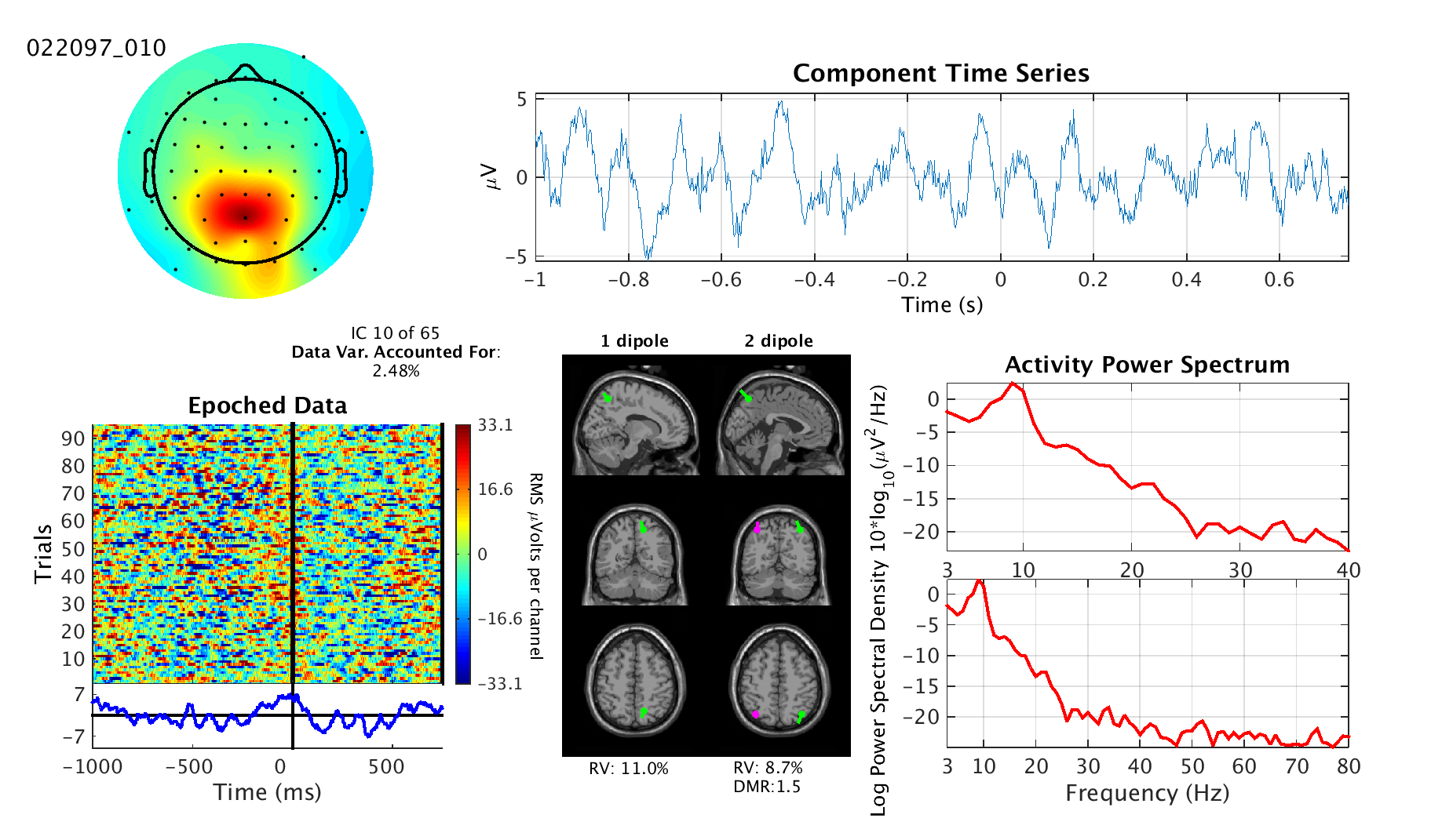
ERP Image (bottom left): The ERP Image shows all the activity of the independent component process across the entire dataset.
ERP stands for "event related potential", which is the repeatable response of the brain to a stimulus. If the dataset
has been "epoched", which means extracting and aligning all relevant experiment trial repetitions, then ERPs can become evident by
taking the average across trials. The average is shown below the ERP Image if the data is epoched. Above the ERP Image,
you can see whether the dataset has been epoched by whether it says "Epoched Data" (epoched) or "Continuous Data"
(not epoched). If the data is not epoched, rather than showing each trial as a row, it will instead show the entire data
folded into a square with the beginning of the recording at the top left and the end of the recording at the bottom right.
Said another way, time progresses smoothly from left to right along the rows, with the higher rows occurring before the lower ones.
Summary:
- Shows the entirety of the component activity in one image.
- If the data has been epoched, a plot below will show the average of all the rows.
-
Component Time Series (top right): This plot shows a segment of activity from the component. While technically
this is duplicate data with that shown in the ERP Image, it provides a clearer view which can sometimes be helpful.
For instance, if you're looking for heart beats or eye movement.
Summary:
- Shows short segment of time series.
- Useful for detecting eye blinks and saccades, heart beats, muscle bursts, and various types of brain waves.
-
Activity Power Spectrum (bottom right): This plot show the power spectrum of the independent component activity
averaged across the entire dataset. To help with scaling, the top plot shows the spectrum from 3 Hz to 40 Hz while
the lower plot shows the spectrum to at most 80 Hz. The spectrum line may stop before 80 Hz if the sampling
rate of the dataset is less than 160 Hz.
The units of the vertical axis are decibels. Be aware that many datasets have line noise contamination
which will cause a peak at either 50 Hz or 60 Hz. Likewise, other dataset may have notch filters at one of those frequencies which
will cause a sharp dip in the spectrum at that frequency. Additionally, the data may have had a low pass or bandpass filter
applied to it which will cause a sharp drop off in power at a seemingly arbitrary frequency. These can be safely ignored
unless the component seems to be predominantly capturing line noise power. See Telling Components Apart
for more information about line noise components.
Summary:
- Shows the component's distribution of power across frequencies.
- Plot is split in two for better scaling of the vertical axis.
- Be aware that filters can cause large dips in power that do not have a physical source.
-
Independent Component (IC) Number and Percent Data Variance Accounted For (middle left):
Percent data variance accounted for describes how much of the original variance in the channel data can be
attributed to this component. Among other things, this measure is useful for determining the relative power
of each component. The component number is the rank of this component after being sorted by the percent data
variance accounted for. The larger the component number and the less power the component accounts for, the less
likely that the component is meaningful. This guideline is not an absolute, but something to be weighed against
other evidence.
Summary:
- Percent data variance accounted for (pvaf) shows the percentage of the channel data accounted for by the component projection.
- Component number can be used (cautiously) to inform how likely it is that the component is meaningful.
-
Image ID (text at the very top/left): This is for our book keeping, so feel free to ignore.
They are formatted as ######_###.
Summary:
- Ignore this.